In many structure-based protein understanding tasks, it is expensive in both time and money to collect labeled data. As a solution, self-supervised pre-training strategies are proposed to acquire informative protein representations from massive unlabeled protein structures. In this tutorial, we will introduce how to pre-train a structure-based protein encoder and then fine-tune it on downstream tasks.

Represent Protein Structure Data

In this part, we will learn how to fetch a structure-based dataset for pre-training and further augment each sample with additional edges to better represent its structure.

Protein Structure Dataset

Let’s first construct a protein structure dataset. For the sake of efficiency, we define a toy protein structure dataset EnzymeCommissionToy based on datasets.EnzymeCommission. Also, we pass two transformation functions into the dataset to truncate overlong proteins and specify node feature.

from torchdrug import datasets, transforms

# A toy protein structure dataset
class EnzymeCommissionToy(datasets.EnzymeCommission):
    url = "https://miladeepgraphlearningproteindata.s3.us-east-2.amazonaws.com/data/EnzymeCommission.tar.gz"
    md5 = "728e0625d1eb513fa9b7626e4d3bcf4d"
    processed_file = "enzyme_commission_toy.pkl.gz"
    test_cutoffs = [0.3, 0.4, 0.5, 0.7, 0.95]

truncuate_transform = transforms.TruncateProtein(max_length=350, random=False)
protein_view_transform = transforms.ProteinView(view='residue')
transform = transforms.Compose([truncuate_transform, protein_view_transform])

dataset = EnzymeCommissionToy("~/protein-datasets/", transform=transform, atom_feature=None, bond_feature=None)
train_set, valid_set, test_set = dataset.split()
print(dataset)
print("train samples: %d, valid samples: %d, test samples: %d" % (len(train_set), len(valid_set), len(test_set)))

EnzymeCommissionToy(
  sample: 1150
  task: 538
)
train samples: 958, valid samples: 97, test samples: 95

Dynamic Graph Construction

The protein data constructed from RDKit only contains four types of bond edges (i.e., single, double, triple or aromatic). Taking the first sample of the dataset as an example, we pick out the atoms of the first two residues and show the chemical bonds between them.

from torchdrug import data

protein = dataset[0]["graph"]
is_first_two = (protein.residue_number == 1) | (protein.residue_number == 2)
first_two = protein.residue_mask(is_first_two, compact=True)
first_two.visualize()

To better represent the protein structure, we seek to dynamically reconstruct the protein graph via the layers.GraphConstruction module. For nodes, we use layers.geometry.AlphaCarbonNode to extract the Alpha carbons from the protein to construct a residue-level graph. For edges, we employ layers.geometry.SpatialEdge, layers.geometry.KNNEdge and layers.geometry.SequentialEdge to construct spatial, KNN and sequential edges between different residues (see Tutorial 3: Structure-based Protein Property Prediction for detailed definitions of these edges).

from torchdrug import layers
from torchdrug.layers import geometry

graph_construction_model = layers.GraphConstruction(node_layers=[geometry.AlphaCarbonNode()], 
                                                    edge_layers=[geometry.SpatialEdge(radius=10.0, min_distance=5),
                                                                 geometry.KNNEdge(k=10, min_distance=5),
                                                                 geometry.SequentialEdge(max_distance=2)],
                                                    edge_feature="gearnet")

_protein = data.Protein.pack([protein])
protein_ = graph_construction_model(_protein)
print("Graph before: ", _protein)
print("Graph after: ", protein_)

degree = protein_.degree_in + protein_.degree_out
print("Average degree: ", degree.mean())
print("Maximum degree: ", degree.max())
print("Minimum degree: ", degree.min())

Graph before:  PackedProtein(batch_size=1, num_atoms=[2639], num_bonds=[5368], num_residues=[350])
Graph after:  PackedProtein(batch_size=1, num_atoms=[350], num_bonds=[7276], num_residues=[350])
Average degree:  41.5771
Maximum degree:  76.0
Minimum degree:  12.0

After such graph construction, we have represented the protein structure as a residue-level relational graph. By regarding spatial edges and KNN edges as two types of edges and regarding the sequential edges of five different sequential distances (i.e., -2, -1, 0, 1 and 2) as five edge types, we derive a relational graph with 7 different edge types. Each edge is associated with a 59-dimensional edge feature which is the concatenation of the one-hot residue features of its two end nodes, edge type, sequential distance and spatial distance.

nodes_in, nodes_out, edges_type = protein_.edge_list.t()
residue_ids = protein_.residue_type.tolist()
for node_in, node_out, edge_type, edge_feature in zip(nodes_in.tolist()[:5], nodes_out.tolist()[:5], edges_type.tolist()[:5], protein_.edge_feature[:5]):
    print("[%s -> %s, type %d] edge feature shape: " % (data.Protein.id2residue[residue_ids[node_in]], 
                                                        data.Protein.id2residue[residue_ids[node_out]], edge_type), edge_feature.shape)

[ILE -> VAL, type 1] edge feature shape:  torch.Size([59])
[TRP -> GLU, type 1] edge feature shape:  torch.Size([59])
[LEU -> GLU, type 1] edge feature shape:  torch.Size([59])
[VAL -> GLU, type 1] edge feature shape:  torch.Size([59])
[ARG -> ASP, type 1] edge feature shape:  torch.Size([59])

Protein Structure Representation Model

TorchProtein defines diverse GNN models that can serve as the protein structure encoder. In this tutorial, we adopt the superior Geometry-Aware Relational Graph Neural Network with Edge Message Passing (GearNet-Edge). In TorchProtein, we can define a GearNet-Edge model with models.GearNet.

from torchdrug import models

gearnet_edge = models.GearNet(input_dim=21, hidden_dims=[512, 512, 512], 
                              num_relation=7, edge_input_dim=59, num_angle_bin=8,
                              batch_norm=True, concat_hidden=True, short_cut=True, readout="sum")

Self-Supervised Protein Structure Pre-training

In this tutorial, we adopt two pre-training algorithms, Multiview Contrastive Learning and Residue Type Prediction, to learn protein representations from unlabeled protein structures.

Multiview Contrastive Learning

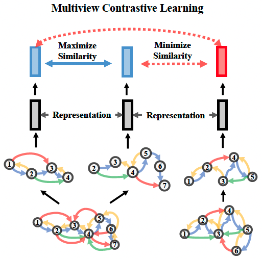
Multiview Contrastive Learning seeks to maximize the similarity between representations of different views from the same protein while minimizing the similarity between those from different proteins. The following figure illustrates the high-level idea of Multiview Contrastive Learning.

We first wrap the GearNet-Edge model into the models.MultiviewContrast module, in which we pass the augmentation functions to use by the aug_funcs parameter and pass the cropping functions to use by the crop_funcs parameter. This module appends an MLP prediction head upon GearNet-Edge. After that, the Multiview Contrast module together with the graph construction model are wrapped into the tasks.Unsupervised module for self-supervised pre-training.

Here we take two different kinds of cropping functions: Subsequence and Subspace. The former randomly takes a shorter consecutive subsequences with length at most 50, while the latter takes all residues within a ball with a randomly selected center residue. After cropping the protein, we randomly choose whether to randomly mask edges in the residue graph as a kind of augmentation.

from torchdrug import layers, models, tasks
from torchdrug.layers import geometry

model = models.MultiviewContrast(gearnet_edge, noise_funcs=[geometry.IdentityNode(), geometry.RandomEdgeMask(mask_rate=0.15)],
                                 crop_funcs=[geometry.SubsequenceNode(max_length=50), 
                                             geometry.SubspaceNode(entity_level="residue", min_neighbor=15, min_radius=15.0)], num_mlp_layer=2)
task = tasks.Unsupervised(model, graph_construction_model=graph_construction_model)

Now we can start pre-training. We set up an optimizer for our model, and put everything together into an Engine instance. It takes about 5 minutes to train the model for 10 epochs on this pre-training task. We finally save the model weights at the last epoch.

from torchdrug import core

optimizer = torch.optim.Adam(task.parameters(), lr=1e-4)
solver = core.Engine(task, train_set, valid_set, test_set, optimizer,
                     gpus=[0], batch_size=4)
solver.train(num_epoch=10)
solver.save("MultiviewContrast_ECToy.pth")

Residue Type Prediction

Residue type prediction is a typical self-prediction task, which masks a portion of residues in the input residue-level graph and seeks to predict the masked residue types according to the context regularities of the protein. This method is also known as masked inverse folding for proteins (predict sequences given structures). The following figure illustrates the high-level idea of Residue Type Prediction.

To perform this task, we wrap the GearNet-Edge model as well as the graph construction model into the tasks.AttributeMasking module, in which an MLP prediction head will be appended upon GearNet-Edge. Note that this module can also be used to pre-train molecule encoders. The module will choose whether to predict atom or residue type according to the view of graphs in the training set.

task = tasks.AttributeMasking(gearnet_edge, graph_construction_model=graph_construction_model,
                              mask_rate=0.15, num_mlp_layer=2)

Now we can start pre-training. Similar as above, we set up an optimizer for our model, and put everything together into an Engine instance. It takes about 8 minutes to train the model for 10 epochs on this pre-training task. We finally save the model weights at the last epoch.

optimizer = torch.optim.Adam(task.parameters(), lr=1e-4)
solver = core.Engine(task, train_set, valid_set, test_set, optimizer,
                     gpus=[0], batch_size=4)
solver.train(num_epoch=10)
solver.save("ResidueTypePrediction_ECToy.pth")

Fine-tuning on Downstream Task

We employ the protein functional terms prediction on the toy Enzyme Commission dataset as the downstream task. This task aims to predict whether a protein owns several specific functions, in which owning each function can be expressed by a binary label. Therefore, we formulate this task as multiple binary classification tasks and seek to solve them jointly in a multi-task learning way. We perform this task using the tasks.MultipleBinaryClassification module which combines the GearNet-Edge model with an MLP prediction head.

task = tasks.MultipleBinaryClassification(gearnet_edge, graph_construction_model=graph_construction_model, num_mlp_layer=3,
                                          task=[_ for _ in range(len(dataset.tasks))], criterion="bce", metric=['auprc@micro', 'f1_max'])

1. Train from scratch

We first evaluate the GearNet-Edge by training from scratch. It takes about 8 minutes to train the model for 10 epochs on this task. We finally evaluate on the validation set.

optimizer = torch.optim.Adam(task.parameters(), lr=1e-4)
solver = core.Engine(task, train_set, valid_set, test_set, optimizer,
                     gpus=[0], batch_size=4)
solver.train(num_epoch=10)
solver.evaluate("valid")

The evaluation result may be similar to the following.

auprc@micro: 0.13146
f1_max: 0.243544

2. Fine-tune the Multiview Contrastive Learning model

We then evaluate the GearNet-Edge model pre-trained by Multiview Contrastive Learning. We initialize the GearNet-Edge with pre-trained model weights. It takes about 8 minutes to train the model for 10 epochs on this task.

optimizer = torch.optim.Adam(task.parameters(), lr=1e-4)
solver = core.Engine(task, train_set, valid_set, test_set, optimizer,
                     gpus=[0], batch_size=4)

_checkpoint = torch.load("MultiviewContrast_ECToy.pth")["model"]
checkpoint = {}
for k, v in _checkpoint.items():
    if k.startswith("model.model"):
        checkpoint[k[6:]] = v
    else:
        checkpoint[k] = v
checkpoint = {k: v for k, v in checkpoint.items() if not k.startswith("mlp")}
task.load_state_dict(checkpoint, strict=False)

solver.train(num_epoch=10)
solver.evaluate("valid")

The evaluation result may be similar to the following.

auprc@micro: 0.184848
f1_max: 0.268139

3. Fine-tune the Residue Type Prediction model

We then evaluate the GearNet-Edge model pre-trained by Residue Type Prediction. It still takes about 8 minutes to train the model for 10 epochs on this task.

optimizer = torch.optim.Adam(task.parameters(), lr=1e-4)
solver = core.Engine(task, train_set, valid_set, test_set, optimizer,
                     gpus=[0], batch_size=4)

checkpoint = torch.load("ResidueTypePrediction_ECToy.pth")["model"]
checkpoint = {k: v for k, v in checkpoint.items() if not k.startswith("mlp")}
task.load_state_dict(checkpoint, strict=False)

solver.train(num_epoch=10)
solver.evaluate("valid")

The evaluation result may be similar to the following.

auprc@micro: 0.176984
f1_max: 0.302019

Note. We observe that fine-tuning the pre-trained model outperforms training from scratch. However, the performance of both schemes are not satisfactory enough, which is mainly attributed to the over small dataset size. We suggest users to perform pre-training on a larger protein structure dataset (e.g., datasets.AlphaFoldDB) to fully investigate the effectiveness of pre-training.

Tutorial 4 - Pre-trained Protein Structure Representations

Represent Protein Structure Data

Protein Structure Dataset

Dynamic Graph Construction

Protein Structure Representation Model

Self-Supervised Protein Structure Pre-training

Multiview Contrastive Learning

Residue Type Prediction

Fine-tuning on Downstream Task

1. Train from scratch

2. Fine-tune the Multiview Contrastive Learning model

3. Fine-tune the Residue Type Prediction model

TorchProtein